This is CDS 2016.

We discussed the format for the course, and the administrative issues thereof. Format for the groups were specified for assignments and the term-project, and the resources residing on the CDS website were pointed out. The computing platform and requirements for the course was defined as well, and installation of R (link), RStudio (link) and Python 2.7.x (link) was recommended.

We discussed the primary goal of the course -- to understand the fundamental notions of Regression, Classification and Clustering on big-data -- with support from techniques like dimensionality reduction. The role of efficient algorithm design was mentioned in this regard, and we started basic discussion on time complexity of an algorithm in terms of different classes of functions and their mutual comparison. Preliminary notions of $\theta$, $O$, $\Omega$, $o$ and $\omega$ in terms of complexity were informally introduced as analogues to 'equality' ($=$), 'less than or equal to' ($\leq$), 'greater than or equal to' ($\geq$), 'strictly less than' ($<$) and 'strictly greater than' ($>$), respectively, in terms of such functions.

  Homework : Plot $f(n)$ against $n$ for various functions $1, 2, 1000$; $\log(n), 2\log(n), 1000\log(n)$; $n, 2n, 1000n$; $n^2, 2n^2, 1000n^2$; $n^3, 2n^3, 1000n^3$; $2^n, 3^n$; etc., and try to observe patterns of clustering, if any, for large values of $n$.

  Lecture Slides   |     Intro to Statistical Learning (ISLR)

We continued our discussion on the basic notions of computational complexity by classifying $f(n)$, the function denoting the time complexity of an algorithm with input size $n$, in various categories -- constant or $O(1)$; logarithmic or $O(\log(n))$; linear or $O(n)$; linearathmic or $O(n\log(n))$; quadratic or $O(n^2)$; polynomial or $O(n^c)$; exponential or $O(c^n)$; factorial or $O(n!)$.

We took a few examples -- addition and multiplication of two numbers (where $n$ is the maximum bitsize of the input numbers), finding the maximum or minimum in a list of numbers (where $n$ is the size of the list), sorting a bunch of playing cards (where $n$ is the number of cards), multiplication of a matrix to a vector (where $m \times n$ are the dimensions of the matrix) -- to illustrate various time complexities.

  Reading : Chapter 3 of "Introduction to Algorithms" (by Thomas H. Cormen, Charles E. Leiserson, Ronald L. Rivest and Clifford Stein)

  Computational Complexity (CS50)   |     Asymptotic Notation (CS50)   |     Complexity Cheatsheet

We motivated the vector-space modelling of data, taking the classic example of representing books as term-frequency vectors on a high-dimensional space, where each term/word represents a new dimension and the values are frequencies of those terms/words in the book. In this context, we learned the notion of distance -- in the sense of norm -- and discussed the three major norms, namely, $l_1$, $l_2$ and $l_{\infty}$.

We tried to analyze the action of a matrix on a vector during multiplication, and figured that an $m \times n$ matrix defined over the reals ($\mathbb{R}$) generally rotates, scales or reflects a vector. We discussed the effect of scaling in terms of the growth of Fibonacci numbers by writing the recurrence relation $F_n = F_{n-1} + F_{n-2}$ in terms of a matrix, and figured that the eigenvalues of this matrix control the scaling.

In fact, we observed that if we decompose a square matrix into its eigenvalues and eigenvectors using the eigen() function in R, then the original matrix can be written as $M = V \Lambda V^{-1}$, where $V$ is the matrix with the eigenvectors of $M$ as its columns, and $\Lambda$ is a diagonal matrix with the eigenvalues of $M$ as its diagonal elements. This gave us the nice relation $M^kv = (V \Lambda^k V^{-1}) v$ for any vector $v$.

We noted that the action of $M$ on a vector $v$ can be naturally decomposed as $Mv = (V \Lambda V^{-1}) v$, which is a three-step process where $V^{-1}$ and $V$ take care of two steps of rotation (being orthonormal matrices), and $\Lambda$ takes care of the entire scaling. We hinted that such a decomposition is possible for any $m \times n$ matrix; it is called the Singular Value Decomposition, computed using the svd() function in R.

  Reading : Lectures 1, 2, 3 of "Linear Algebra" by Gilbert Strang (link)   |   "Geometric Review of Linear Algebra" by Simoncelli (link)

  Linear Algebra (Gilbert Strang)   |     Fibonacci and Eigenvalues (Anstee)   |     Linear Algebra Review (Savov)

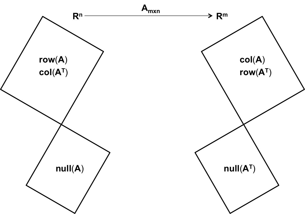
In this lecture, we tried to view an $m \times n$ matrix as a linear operator (analogous to a function) from $\mathbb{R}^n$ to $\mathbb{R}^m$, and attempted an analysis of matrices in terms of linear functions. We learned the notions of linear dependence and independence of a set of vectors, and tried to view, geometrically, the span of a collection of vectors as the space generated by taking their linear combinations. Using the notion of span, we tried to identify the range of the matrix as a subspace of $\mathbb{R}^m$, and figured that the range of an $m \times n$ matrix as a linear operator is essentially its column space, that is, the span of its column vectors. Evidently, $\dim(\textrm{col}(A_{m \times n})) \leq m$.

It seemed quite natural to look at the $n \times m$ matrix $A^T$ as a linear operator from $\mathbb{R}^m$ to $\mathbb{R}^n$ (it is NOT the inverse operator of $A$). It was immediately obvious that the row space of the matrix $A$ is identical to the column space of $A^T$, that is, $\textrm{row}(A) = \textrm{col}(A^T)$. Thus, we concluded that $\dim(\textrm{row}(A)) = \dim(\textrm{col}(A^T)) \leq n$, and that $\textrm{row}(A)$ is a subspace of $\mathbb{R}^n$.

Next, we viewed the operation of the matrix $A$ on a vector $v \in \mathbb{R}^n$ as a collection of dot products of the rows of $A$ with $v$, and concluded that the solutions of $Av = 0$ must all be orthogonal to every row of $A$, and hence, must be orthogonal to $\textrm{row}(A)$. The collection of all such vectors is called the null space of $A$, and the above analysis illustrated that $\textrm{null}(A) \perp \textrm{row}(A)$. We also observed that $\textrm{null}(A)$ is non-empty as it always contains the zero-vector ($0$) in $\mathbb{R}^n$, and that $\dim(\textrm{null}(A)) \leq n$. Similarly, we identified the null space of $A^T$ as a subspace of $\mathbb{R}^m$, and observed that $\textrm{null}(A^T) \perp \textrm{row}(A^T)$, that is, $\textrm{null}(A^T) \perp \textrm{col}(A)$.

In effect, we identified four subspaces for the $m \times n$ matrix $A$ in this lecture -- the row space of $A$ (same as the column space of $A^T$), the column space of $A$ (same as the row space of $A^T$), the null space of $A$, and the null space of $A^T$, as shown in the figure below.

  Reading : Paper 1 and Paper 2 by Gilbert Strang   |   "Geometric Review of Linear Algebra" by Simoncelli (link)
  Homework : Determine the dimensions of all the four subspaces identified in this lecture, and find their relationship with $m$ and $n$.

  Linear Algebra (Gilbert Strang)   |     Paper 1 (Gilbert Strang)   |   Paper 2 (Gilbert Strang)   |     Linear Algebra Review (Savov)

Introduced linear regression from the notion of solving linear equations. Detailed abstract and further resources to come.

Introduced the gradient descent algorithm to solve the problem of linear regression. Detailed abstract and further resources to come.

Discussed the batch gradient descent and stochantic gradient descent algorithms to solve the problem of linear regression. Detailed abstract and further resources to come.

Discussed the hypothesis testing and parameter estimation point-of-view of linear regression, in terms of estimating the underlying linear model in data. Detailed abstract and further resources to come.

Discussed the singular value decomposition and principal component analysis in connection with explaining variance in the data. Detailed abstract and further resources to come.

Introduced the notion of classification as another supervised learning problem, and discussed decision trees as a model for solving the problem. Detailed abstract and further resources to come.

Introduced the notion of random forests as an ensemble model based on decision trees, in connection with solving the problem of classification. Detailed abstract and further resources to come.

This was a Lab Session, involving hands-on application of linear models and tree-based models to a dataset. Discussed variable importance factor obtained from random forests. Detailed abstract and further resources to come.

Discussed (recap) various notions of distance, and introduced the concept of nearest neighbor search in context of text-documents. Introduced TF-IDF for documents, and kd-Tree as a data structure for efficient neighborhood search. Detailed abstract and further resources to come.

Introduced the concept of unsupervised learning and discussed various algorithms for clustering data points. Specifically, discussed k-Means and hierarchical clustering algorithms and their usage. Detailed abstract and further resources to come.

We had a wonderful guest lecture by Bodhisattwa, Robin, Ayan and Jayanta (from the PGDBA senior batch), introducing the concept of neural networks and deep learning in context of their participation and experience in the Data Science Game 2016. Detailed abstract and further resources to come.

Discussed the concept of bias-variance tradeoff in context of overfitting and underfitting a model to a given dataset. Introduced regularized models like ridge regression and lasso to illustrate the optimization of bias and variance. Detailed abstract and further resources to come.